Research Article Online Published: 10 Feb 2026
Arch Appl Sci. 2026; 1(1): 23-42 doi: 10.5455/AAS.20250818034145 Predictive Analysis of Rainfall using Supervised Machine Learning Algorithms Joshua Ayodeji Oluwatola, Olusola Olajide Ajayi, Ayomide Moses Oluwatola. Abstract Aim/Background The study highlights the significance of rainfall in Earth's water cycle and its impact on ecosystems and human activities. Stating why unusual rainfall conditions can threaten food security and livelihoods, necessitating early warning systems for adaptation. It explores the historical evolution of weather prediction efforts from some ancient theories to modern machine learning (ML) techniques. This study then compares four supervised machine learning algorithms, Random Forest (RF), Long Short-Term Memory (LSTM), Autoregressive Integrated Moving Average (ARIMA), and Linear Regression (LR), to forecast daily rainfall amounts across 49 Australian cities using a 2007–2017 dataset downloaded in 2022. Methods Missing data were addressed through a hybrid procedure combining a custom algorithm with K-Nearest-Neighbor imputation, and mode imputation for categorical fields. Model performance was evaluated using MAE, MSE, and RMSE over forecast horizons (1, 5, 10, 15, 20, 25, and 30-days interval) and compared to a naïve zero-rain baseline. Categorical inputs for neural models were converted to learned embeddings; LR used feature selection informed by Pearson correlation and predictors were scaled where appropriate; RF training omitted scaling; ARIMA was trained and validated using walk-forward validation on a single long station record; ML models were trained across multiple stations with an 80/20 train/test split. Results Results show that the zero baseline is a strong MAE benchmark due to heavy zero-rain inflation (median rainfall is 0 mm); no single learned model outperformed it on MAE across all horizons. ARIMA consistently reduced squared-error metrics (MSE & RMSE) and per-formed competitively on MAE, indicating its strength at capturing large events and short-term temporal structure. RF and LR produced moderate errors overall, while LSTM yielded competitive MAE but substantially larger MSE/RMSE – suggesting occasional large outliers. Errors are geographically and seasonally heterogeneous (largest in Dec–Mar and at tropical stations such as Darwin). Results are partially affected by preprocessing and validation differences (notably ARIMA’s single-station training versus ML models trained on multiple stations). Conclusion Forecasting daily rainfall from routine meteorological predictors on this multi-location dataset is challenging because of zero-inflation and spatial heterogeneity. A single-stage regression that only minimizes MAE is insufficient for operational use. Recommended next steps include two-stage occurrence + amount modeling, consistent per-location temporal splits for fair model comparison, climate-zone or location-specific models to better capture local patterns, and conditional evaluation on wet days and extremes. Key words: Rain Prediction, Random Forest, ARIMA, LSTM, Linear Regression, Machine Learning, Missing values   ARTICLE TOOLS Abstract PDF Fulltext How to cite this article Citation Tools Related Records   Articles by Joshua Ayodeji Oluwatola Articles by Olusola Olajide Ajayi Articles by Ayomide Moses Oluwatola on Google on Google Scholar

Introduction

Rain in itself is droplets of liquid water that form when atmospheric water vapor condenses and becomes heavy enough to fall under gravity. It plays a crucial role in the hydrologic cycle, as rain contributes significantly to the replenishment of Earth’s fresh water. It creates suitable conditions for diverse ecosystems and supplies water essential for hydroelectric power generation and agricultural irrigation [1]. However, when rainfall patterns become irregular, it can lead to unpredictable seasons, erratic rainfall, unexpected weather occurrences, or even the disappearance of transitional seasons. These changes could have profound effects on food security, disrupt the livelihoods of countless people, and influence the migration choices of atrisk communities [2]. Moreover, Earth’s climate is changing, with rising temperatures, changes in snow and rainfall patterns, and an increase in severe weather occurrences like heavy rainstorms and recordbreaking temperatures. A significant portion of this is tied to the elevated levels of CO2 alongside other greenhouse emissions in our atmosphere, predominantly caused by human activities [3]. For these reasons, it is advisable to be ready for any form of inconvenience that may occur due to unusual rainfall patterns. To accomplish this, predicting rainfall holds significant importance [4]. In retrospection, the earliest known attempts towards predicting weather were made by Babylonians at about 650 B.C. In an effort to forecast weather changes in the near term, they were examining cloud patterns and optical effects such as halos. About 310 years later, the Greek philosopher Aristotle authored “Meteorologica,” a philosophical work that presented theories on how rain, hail, clouds, wind, hurricanes, lightning, and thunder occur. His observations concerning the weather were deeply perceptive, but as a result, they contained some significant errors. Even though there were errors, his theories were considered fact by many for about 2000 years, as there was no other generally accepted theory. It was not until the 17th century that many of his theories were challenged and eventually disproven. By 300 B.C., the Chinese had created a calendar derived from their weather observations, dividing the year into 24 festivals, each linked to a distinct type of weather. In the Renaissance period (15th and 16th centuries), there were several inventions that allowed the measurement of some atmospheric features like humidity of air, temperature, and atmospheric pressure [5].

Consequently, with the development of new instruments, more robust measurements of the atmosphere began. Weather conditions could then be monitored better thanks to various instruments such as the telegraph and radiosnode. These instruments are still used to record weather conditions today, making more data available for observationbased weather forecasting [6]. Be that as it may, the importance of rainfall prediction has increased due to its intricate nature and essential uses such as flood prediction and tracking pollutant concentrations. Traditional approaches often rely on complex statistical models that can be computationally expensive and budgetintensive, or they may not be applied effectively to downstream applications. As a result, researchers are exploring alternative methods that combine machine learning (ML) algorithms with timeseries data to tackle these challenges [7].

Research gap and contribution

Although many studies have explored rainfall prediction using traditional statistical or singlemodel approaches, few have systematically compared both statistical [Autoregressive integrated moving average (ARIMA), linear regression (LR)] and modern ML [random forest (RF), long shortterm memory (LSTM)] techniques on the same dataset with explicit consideration of dataimputation bias. Moreover, limited attention has been given to evaluating model behavior across different forecast horizons and rainfall intensities. This study bridges that gap by (i) implementing a unified multimodel framework, (ii) integrating a reproducible hybrid imputation method, and (iii) analyzing model robustness under varying rainfall magnitudes and temporal windows. The resulting benchmark provides both methodological transparency and practical insight for environmental data scientists and meteorological agencies.

Related works

Paras [8] conducted a study on weather forecasting using multivariate linear regression. The study was conducted with data recorded at a local station for a 3-year period. The input data was averaged from daily recordings over weekly intervals, and rainfall amounts were classified into five groups: very low, low, medium, high, and very high. The study evaluated three periods: 15, 30, and 45 weeks. Of the time frames tested, the period of 15 weeks proved to be the most suitable for prediction. In the same year, [9] conducted a study on monthly rainfall estimation using various models. It was conducted with data recorded across four weather stations in the study area over a 41-year period. The data used as input consisted of monthly rainfall measurements recorded at the stations. Of the models developed, multilinear regression was the best for the task, which achieved a relative error of 0.7%, indicating its potential utility in rainfall prediction. About 2 years later, [10] carried out a study on yearly rainfall using ARIMA, FST, and the Theil-Sen estimator with time series data spanning a 31-year period. The models’ forecasting prowess was evaluated using mean absolute error (MAE), Root mean squared error (RMSE) and R2, with FST outperforming the other models on all metrics, demonstrating its effectiveness as a reliable tool for yearly rain prediction. A study on the application of support vector regression (SVR) for the prediction of rainfall was carried out by [11] 1 year later. The study proposed the development of separate models for forecasting the amount of rain, max., and avg. rain, each model included three submodels for 1-, 7-, and 10-day forward forecasting. The models were trained with rainfall data spanning a period of 6 years (from Mar. to Oct. annually). Key features included date, min., max., avg., total, and moving average, date being the id, max. the maximum rainfall, min. the minimum rainfall, and avg. being the average rainfall. The models were evaluated using RMSE and MAE. The results showed that the 1-day ahead proposed submodel’s prediction was closest to the actual rainfall data. In order to predict rainfall in Malaysia, [12] evaluated the effectiveness of multiple ML classifiers [support vector machine (SVM), Naïve Bayes, neural network, decision tree (DT), and RF) in carrying out the task, using rainfall data spanning a 4-year period. The features used were: temperature, river movement, rain amount, humidity, and water depth. Feature selection was not performed, and the mean average was used to fill in missing data. Accuracy (%) at different dataset splitting was used to evaluate the models, of which random forest (RF) performed best. In [13], the authors used a modified version of linear regression (LR) for rainfall prediction, with data spanning a 102-year period. The features used were rainfall, temperature, and cloud cover. Tharun et al. [14] conducted a study on predicting rain amounts in Coonoor. The model was trained using daily recorded parameters such as temperature, wind speed, cloud speed, humidity, and wind direction. Rainfall intensities from nearby stations within a 7 km2 area were also included to make the model more efficient. Various regression models, SVR, RF, and DT were compared. The models were evaluated based on R2 and Adjusted R2 values, with which the RF model was found to be more efficient and accurate compared to the other models compared. Vijayan et al. [15] employed ML algorithms such as RF, DT, and SVM to classify rainfall. The models were trained and tested using 12 years of historical weather data. RF achieved the highest accuracy of 96.447%. In Liyew and Melese’s work [16], environmental features fed into the models were chosen using Pearson correlation. RMSE and MAE were used to measure their performance.

Research methodology

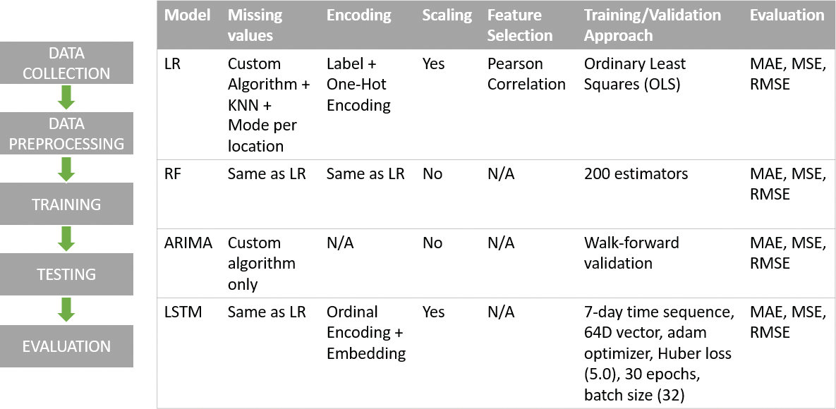
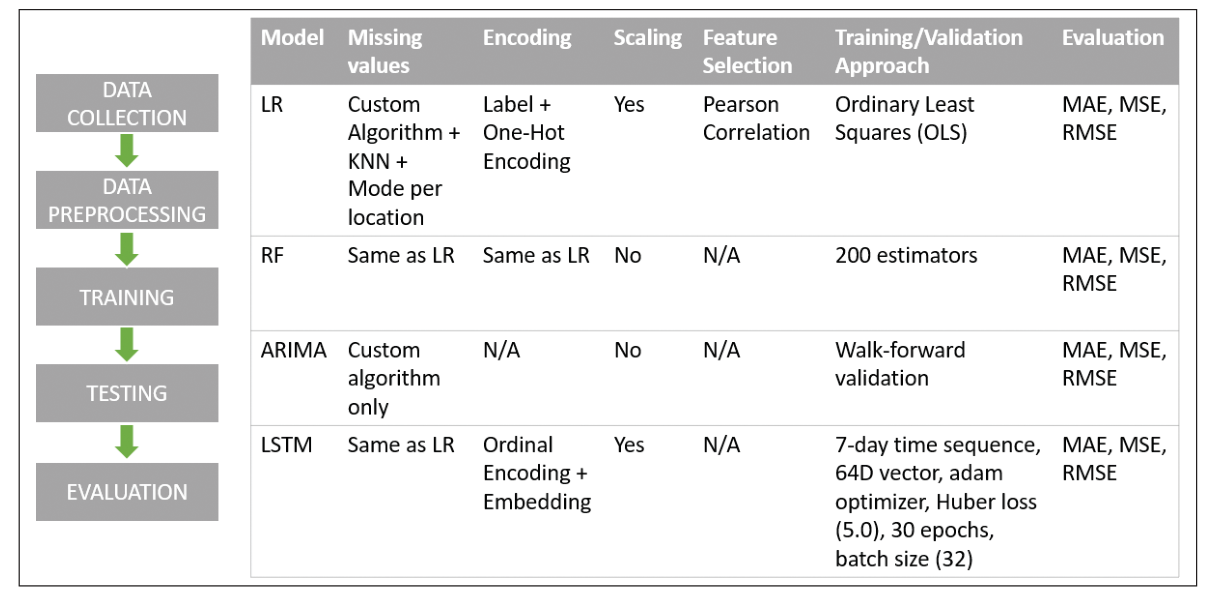
In this study, a dataset containing rainfall data and meteorological parameters observed over a 10-year period across 49 cities (downloaded in the year 2022) was used to train and test the models. It used an algorithm to fill missing values, when the algorithm was not sufficient k-Nearest Neighbor (KNN) imputer was used; categorical missing values were filled with the mode in the location (this series of steps was used in handling missing values for all but the ARIMA model where the algorithm alone was sufficient), and created new columns that contained the shifted rainfall data (for models that required it). For the Ordinary least squares LR model, features that had some degree of correlation to the predictand were discovered using Pearson’s correlation matrix, the dataset was then trimmed to contain only these features; the predictors in the dataset were scaled (as they had different units); categorical features were converted into numerical form using a combination of Encoding techniques (this step was done for the applicable models, except LSTM, where embeddings were used after the encoding). The dataset was split 80–20, 80% of the dataset for training, 20% for testing (this same ratio was used for all models). The predictors and predictands were then specified. Evaluating metrics were then used to assess performance. Correlation and Scaling were not performed for the RF models. The RF models were instantiated with 200 estimators. For ARIMA, it was ensured that there was no missing date in each location’s date range; the models were trained with data from the location with the most data (had 115 months data – about 10 years); walkforward validation was employed to get its forecast across multiple points to compute its evaluation metrics. Whereas with LSTM, numerical predictors were scaled; a sequence of 7 days, grouped by location and sorted by date, was created, time varying and fixed features, in each sequence, were treated differently; embedding dimensions were calculated based on the number of unique features in each categorical column. See the hybrid visual in Figure 1, which summarizes how this research was undertaken. The analysis spanned the years 2023–2025.

Methodological Details

Data collection

In the data collection stage, data in a commaseparated values (csv) file compiled by Joe Young and Adam Young was downloaded from kaggle.com. This same base data was used for all models, whereas the next stages differ across models.

Data preprocessing

Missing values

Different techniques, as outlined below, were used to address the missing data issues. The custom algorithm, which was used by all models, was implemented to fill null values and is shown in Algorithm 1.i. Selected replacement: Null values were replaced with values from the nearest available city (weather station), determined by their geographical location’s distance, recorded on the same day. This was implemented in the custom algorithm.

ii. Selected averaging: In cases where the null value (atmospheric feature) was also not recorded in the closest city on the same day, the value recorded in at least four of the five closest cities on the same day was averaged and used to fill the null value. In cases where this was also insufficient, an average of the values recorded in the week the null value was found – in the same city, was used to fill the null value. This was also implemented in the custom algorithm.iii. KNN imputing: In cases where the above techniques (custom algorithm) were insufficient, the KNN imputer was used. This was used for the LR, LSTM, and RF model.iv. Mode imputing: For the categorical data, the mode in each location was used to fill the missing value per location. This was also used for the LR, LSTM, and RF model.

Linear regression

As some data, such as rainfall amount of the next day and month was not available in the dataset but could be insinuated from the available data, columns were added that contained these data, involved shifting the dataset by the required periods forward, for rainfall amount of the next days; To select features to be used as predictors, Pearson’s correlation was used to identify features that have direct or linear correlation with the predictands (feature extraction) as it was used in related works reviewed; Categorical

data were translated into numerical form because the LR model can only take in numerical data: they were translated using label encoding (LE) and onehot encoding (OHE) technique.i. LE: This is a commonly used encoding technique for handling categorical data. It works by sorting the variables alphabetically (unless explicitly specified otherwise) and then representing the sorted variables with positive integers – for an example of how it works [17]. Because ML models may assume there is a rank – when there isn’t, it is ideally only suitable for categorical data with only two variables or categorical data with ranked variables [18].ii. OHE: This is a widely used encoding technique when working with categorical data in ML. It works by converting categorical values into numeric vectors that ML models can understand – for an example of how it works [19]. It is most suitable when there is no order or priority among the categories [20], but it can lead to increased dimensionality and sparsity as categories increase [21].One of the categorical features (RainToday) was encoded using LE, while the others were encoded using OHE, both LE and OHE were facilitated by the corresponding classes bundled with scikitlearn. The categorical features in the dataset were: location, wind gust direction, wind direction at 9 am, wind direction at 3 pm, and rain that fell today (on the date). All predictors were scaled.

Random forest

Had almost the same preprocessing steps as LR, the differences were: no correlation was done to determine features to be used as predictors, all features, except the date (month was extracted and used) and rainfall amount, were used as predictors, and one categorical feature (month, that was insinuated from date) was encoded using radial basis function (RBF), which is better than One-Hot and Cyclical encoding technique in encoding time data (cyclical in nature), especially when it’s going to be fed into treebased models [22]. An RBF is a Algorithm 1: Handling missing values 1:Begin 2:Import libraries 3:Import dataset 4:Read dataset 5:For each row in dataset do 6: If no value is detected (Na) in one column then 7: Check if corresponding missing value is available in nearest city 8: If available then 9: Fill with the value recorded on the same day from the nearest city 10: Else 11: Check for the missing value recorded in the 5 nearest cities 12: If available in at least 4 of the cities then 13: Compute the average and use to represent missing value 14: Else 15: Compute the average value recorded in the week and use to replace missing value 16: End if 17: End if 18: End if 19:End for 20:End

realvalued function whose output depends only on the distance between the input and a fixed point (often called a center), which can be represented as: φ(x)=φ ̂(||x - c||), where c is the center, x is the input, and φ is the function. Typically, the Euclidean distance is used, which means the function’s value changes only based on how far x is from some center c [24]. When working with cyclical or periodic

timeseries features, like month of the year or day of the week, standard numeric encoding can mislead the model, as for example, encoding day of the week as something like 0–6 (0 – Monday, and 6 – Sunday), might make the model believe Monday is farther to Sunday than Wednesday. RBF addresses this by representing each time pivot via multiple RBFs, each centered at different points in the cycle. These RBFs effectively reveal how close a time point is to certain key positions in the cycle [25].

Autoregressive integrated moving average

As ARIMA is a timeseries model, it requires a date column and a column containing the data to be predicted, so it cannot take in data from different locations that had the same date. For this reason, the options were to choose one or more locations or use ARIMA for all locations individually. This study went with choosing one location – the location with the most data and fewest missing values. Also, because the model assumes the time series is evenly spaced, i.e., one reading per day, it was made sure that missing dates in the location in the dataset were added.

Long shortterm memory

Categorical features were first encoded using Ordinal Encoding (an encoding technique that seems similar to LE, except it assigns numerical values based on perceived order, instead of arbitrarily [26]), before being fed into Embeddings – a

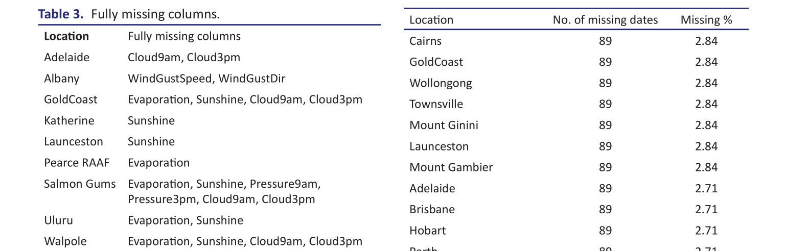
Witchcliffe Evaporation, Sunshine, Cloud9am, Cloud3pm

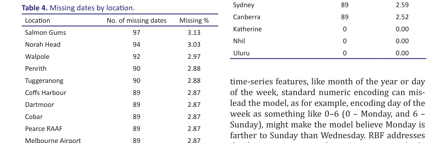
Melbourne Airport892.87 Mildura892.87 Norfolk Island892.87 Richmond892.87 Sale892.87 Sydney Airport892.87 Wagga Wagga892.87 Badgerys Creek892.87 Woomera892.87 Witchcliffe892.87 Watsonia892.87 Williamtown892.87 Portland892.87 Nuriootpa892.87 Moree892.87 Perth Airport892.87 Newcastle892.85 Alice Springs892.84 Albany892.84 Ballarat892.84 Bendigo892.84 Albury892.84 Perth892.71 Melbourne892.71 Darwin892.71

v is the number of unique entries in a feature’s column.

Training and testing

Across all models, 80% of the dataset was used for training and 20% for testing (except for ARIMA, which started at the 80–20 split but increased along the line).

Linear regression and Random forest

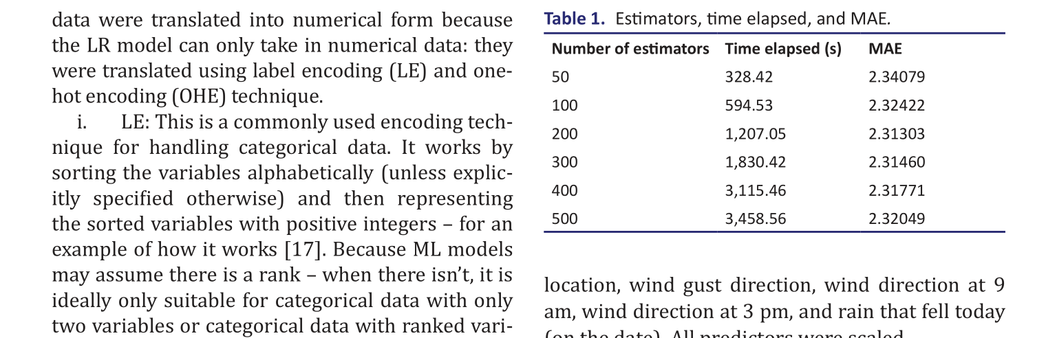
The LR models were trained on the scaled training data and tested with the test dataset, whereas the RF models were trained on the unscaled training data using 200 estimators, chosen based on hardware limitations and tiny difference in performance – Table 1 for the number of estimators, MAE, and time it took to train. Likewise, it tested with the test dataset.

Autoregressive integrated moving average

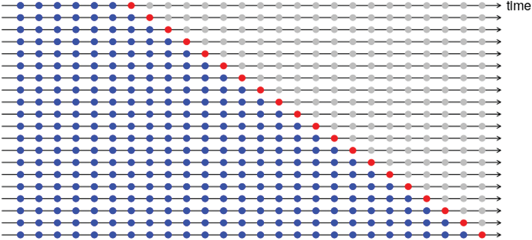
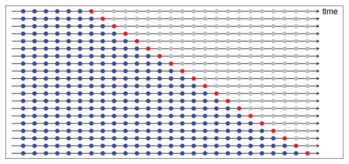
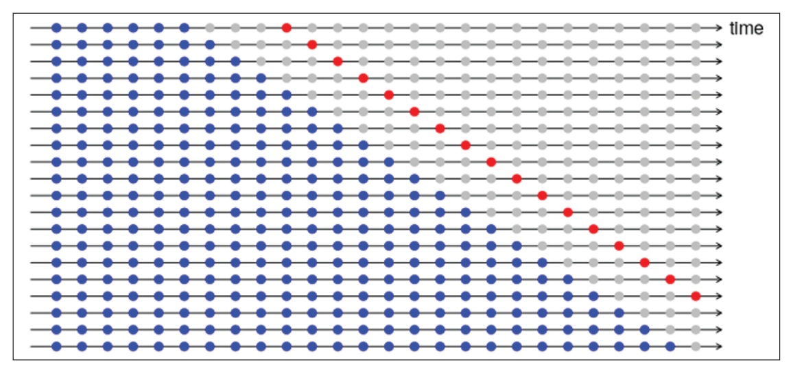
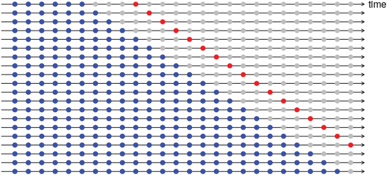
This study adopted an approach called walkforward validation (also known as timeseries crossvalidation) for the ARIMA models. This approach was chosen because it provides average evaluation metrics across the test set, rather than relying on a single traintest split, which may lead to biased results due to the arbitrary choice of the split point. Walkforward validation generates multiple splits across the time period, with the training set increasing at each iteration. Figures 2 and 3 illustrate this process (where the blue dots represent the training set, red dots represent the test set, and each line denoting an iteration). In this study, the initial split was made at 80% of the dataset. At each iteration, the prediction of an interval and its true value was stored. The training set was subsequently expanded, with a step of 1, and the process was repeated until predictions were obtained for the entire test set.

Long shortterm memory

The model architecture incorporated three types of inputs: (i) sequential numerical features, (ii) sequential categorical features, and (iii) static categorical features.For categorical inputs, an embedding layer was applied. Sequential categorical features (features that change per step, in a sequence) were embedded and concatenated with the numerical timeseries inputs, while static categorical features were embedded separately and concatenated with the LSTM output. The concatenated representation was passed through a 64-unit LSTM layer, followed by dense layers (32 units with ReLU activation), and finally a singleunit dense output layer with a linear activation for regression.The model was compiled using Adam optimizer, with the Huber loss function of 5.0 (5.0 was used as it is around the 90th percentile, which was 6.2 mm) to mitigate sensitivity to outliers, and MAE as an evaluation metric. Training was done for 30 epochs with a batch size of 32. A ModelCheckpoint callback was employed to save the bestperforming model based on the lowest validation MAE. After training, the model was tested on the test set using the saved best model.

Evaluation

Here, three metrics that gauge the difference between the model’s forecasted values and the actual outcomes were used to assess the forecast: i. MAE: This metric is commonly applied in evaluating the performance of a regression model. It is calculated as the mean of the absolute differences between the forecasted values and the observed data. MAE’s formula is:

n (n-1)

Where:n represents the total amount of observations inside data collection,ai represents the observed data at the i-th observation,bi represents the forecasted value at the i-th observation,| | denotes the absolute value of the expression within the brackets, Σ indicates the sum of the differences from the first term to the nth term.A lower MAE indicates superior performance. MAE is very useful in cases where errors are evenly spread, and extreme outliers are absent – since it is not sensitive to the presence of outliers [29].ii. Mean squared error (MSE): Computed by subtracting the forecasted and actual values, squaring this difference, and then averaging the results. A larger MSE means that the data points are more widely dispersed from the average, suggesting greater variation or discrepancy among the data points. A lower MSE implies that the data points are clustered more closely around the mean, indicating less variation and fewer errors. As expected, a lower mean squared error is preferred because it indicates that the data points are tightly grouped around the mean, reflecting fewer errors and a more accurate model [30].The meansquared error is calculated using the following formula:

(n-1) where, ∑, n, ai, and bi mean the same as specified for MAE above. iii. RMSE: Works by taking the square root of value obtained from the MSE function. Like mean squared error, it measures the spread of observations around its mean. However, because it involves taking the square root, it is a more interpretable

measure (it normalizes the error back to the same unit as the original values) and it penalizes larger errors more heavily [31].

RMSE is calculated using the following formula:

n where, ∑, n, ai, and bi mean the same as specified for MAE above Implementation, Results, and Analysis The study made use of the Python programing language and some of its libraries used for data analysisrelated tasks.

Implementation working environment

The working environment was powered by Anaconda, a popular distribution of Python for data sciencerelated tasks, it typically comes bundled with other libraries and tools, and more specifically, Jupyter Notebook, which accommodates multiple programming languages, such as Python [32]. Table 2 shows the exact version of required application software the study used; The study was carried out on a 6 GB RAM (1333 MHz) Intel core i3 (2328 M 64 bit) laptop initially, but in later revisions, it was carried out on a 16 GB RAM (2400 MHz) Intel core i5 (8365 U 64 bit).

Implementation Results

Data preprocessing

Missing values

Linear regression, RF, and LSTM The dataset contained 343,248 entries that contained null values, about 10% of the total entries in

the dataset. The algorithm written to handle missing values was implemented with python, but it was only able to reduce missing values from 343,248 to 342,740 entries. Prior to grouping the dataset by location before using KNN imputer (to ensure it only uses nearest neighbors in the same location), it was discovered that some locations had null values for some features (i.e., those features were not available in the locations). See Table 3 for the breakdown. These locations were dropped from the dataset, though we considered dropping only locations with more than two features that were not available, and filling with the data recorded on the same day in the closest city (or 3 days interval), but we did not want to risk blurring localized weather behavior. After dropping rows with these cities’ data, the missing values in the dataset reduced to 232,467 entries (however, the total entries in the dataset reduced by 18.9%). KNN Imputer was then used with five nearest neighbors, which reduced the missing entries to 23,872 entries, which were the missing categorical entries that KNN imputer was not used to fill (the imputer can only work with numerical values). These categorical entries were then filled with simple imputer with the strategy: most frequent. It used the most frequent entries in the location where the missing value was found, which then resulted to zero null values in the dataset. It is important to note that even after dropping some rows (where some features were completely unavailable), about 8.5% of the dataset still contained missing values across various numerical and categorical features. While we employed a threestage, locationaware imputation strategy carefully designed to minimize distortion by respecting spatial and temporal locality (using samecity and date information), avoid global averaging or arbitrary filling that can bias models, and preserve important locationspecific patterns, it is important to acknowledge that imputed values may still lack the variability of true observations, models may become

overconfident in patterns that were artificially filled, and performance metrics should be interpreted with caution, especially for rare weather events.While the multistage imputation strategy significantly reduced missing entries without oversimplifying spatial patterns, the approach may slightly underestimate extreme values. Consequently, performance metrics should be interpreted with awareness of possible bias introduced by synthetic filling.

ARIMA model

The dataset originally contained 3,261 missing rainfall values, but after ensuring there were no missing dates in each location (involved adding missing dates in the dataset, as ARIMA assumes the time series is evenly spaced, i.e., one reading per day), this number increased to 7,373 missing rainfall values – about 5% of the total rainfall values (See Table 4 for the breakdown of how many missing dates were found in each location). These missing rainfall values were then filled with an implementation of Algorithm 1.

Feature addition

Linear regression and RF regression model

Seven features were added to the dataset (excluding the ones introduced with OHE), namely: Rain_1day_after, Rain_5day_after, Rain_10day_after, Rain_15day_after, Rain_20day_after, Rain_25day_after, and Rain_30day_after. In addition, features were added as a result of RBF encoding, for RF models.

Feature selection

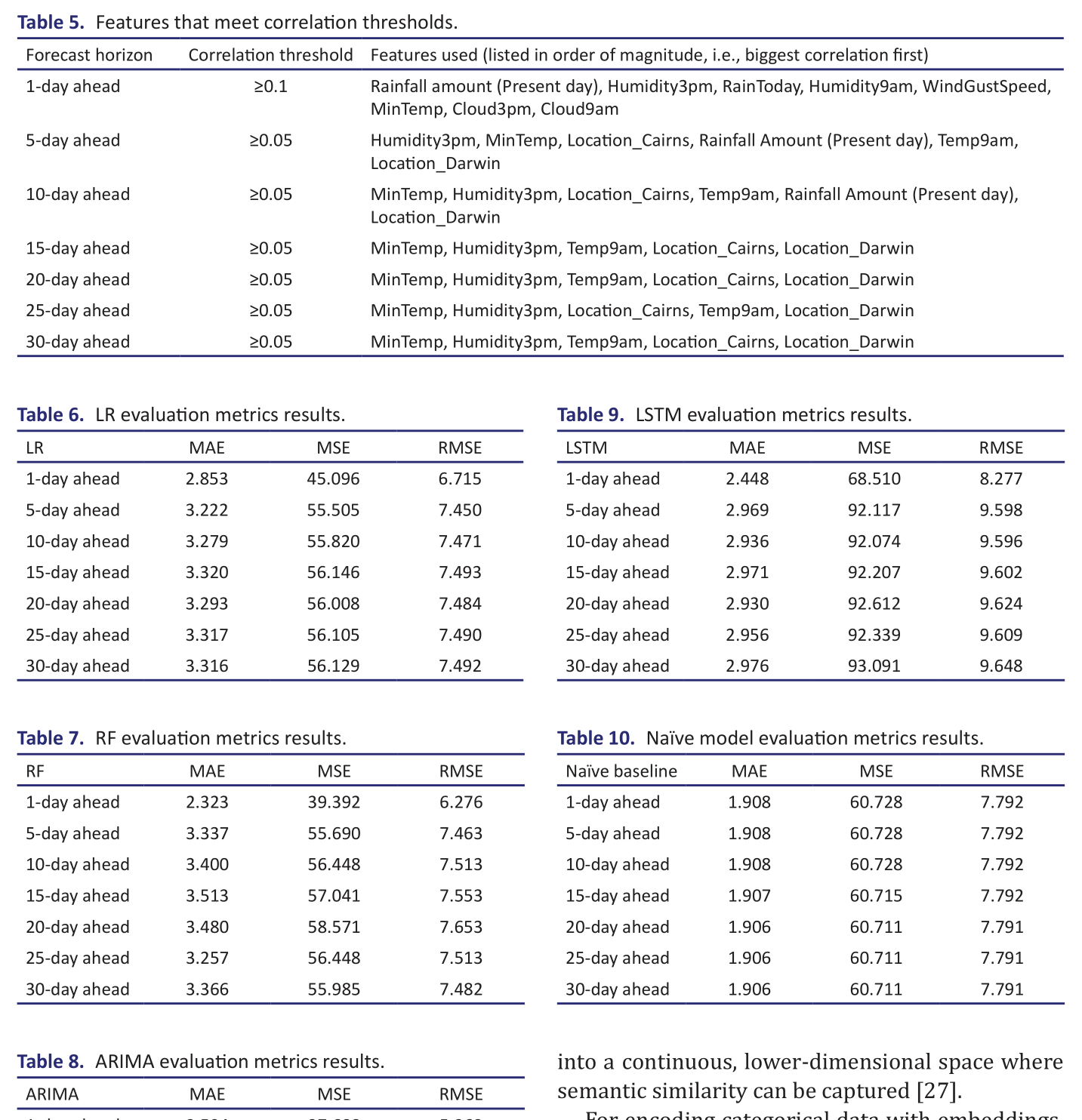
Table 5 shows the correlation threshold and features that met the threshold for all forecast horizons. It can be observed that rainfall amount on the present day only had a linear correlation with 1-, 5-, and 10-day ahead rainfall amount. Whereas humidity at 3 pm and minimum temperature observed in the day, had a correlation on all forecast horizons (strongest on

all but the 1-day ahead horizon), and features like Location_Cairns and Location_Darwin (features introduced with OHE, that indicates whether it is those locations or not) had a correlation across all but one forecast horizon – 1-day ahead – despite them not being the locations with the most features.

Training stage

Linear regression and RF regression model

Both the LR models and the RF models were implemented using scikitlearn library. For RF, seven models were instantiated and trained for the seven predictands. Each with 200 estimators, with other parameters being default, and split in an 80–20 fashion. Whilst for LR, seven models were also instantiated and trained for the seven predictands, but each with their corresponding selected features, using default parameters.

ARIMA and LSTM

The ARIMA models were implemented using the auto_arima method from the pmdarima library. This method performs a search over several model parameter combinations and selects the model with the minimal akaike information criterion score. For this study, the seasonal parameter was set to False (it was set to True to test for seasonality in the training dataset, but it defaulted back to False during training), and stepwise was set to True.As ARIMA cannot handle multiple location data (i.e., dataset where the same dates may occur multiple times), models were trained with timeseries data observed in one selected location, selected as thus: because it had the medium number of missing dates and highest data available (Canberra). Initially, the data was split in an 80–20 fashion, where the training data was 80%, walkforward validation was then used to get the predictions at multiple points in the time series (with a step of 1). Stepwise search was performed to choose the optimal parameters for the ARIMA models.

While the LSTM models were implemented using the Tensorflow/Keras framework, with the approach specified in methodological details.

Evaluation stage

In this stage, a naïve baseline model was added, which predicts 0 mm every day, and compared to

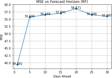
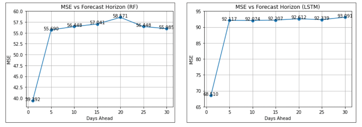
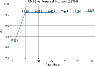
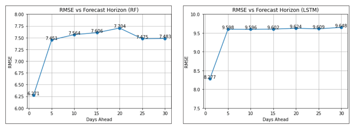
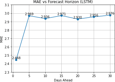
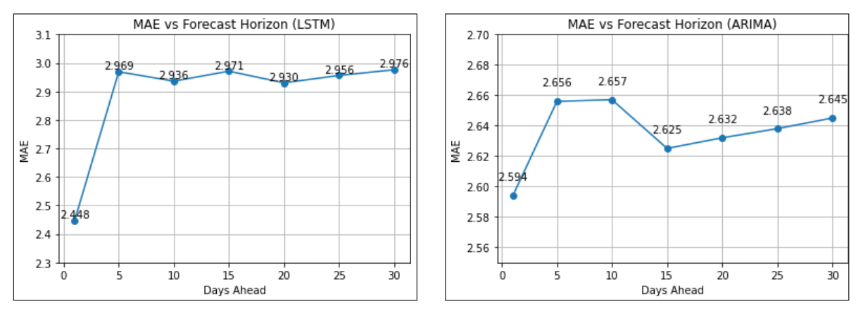
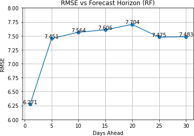
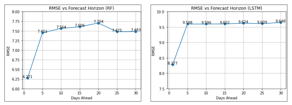
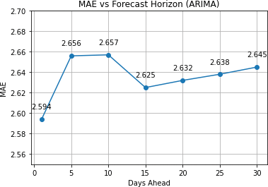
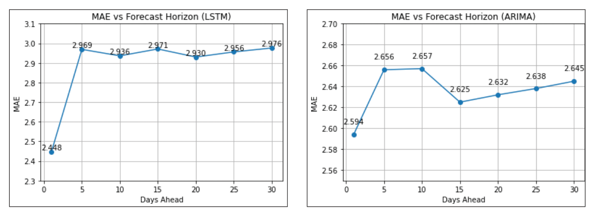
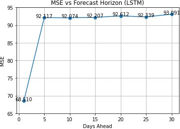
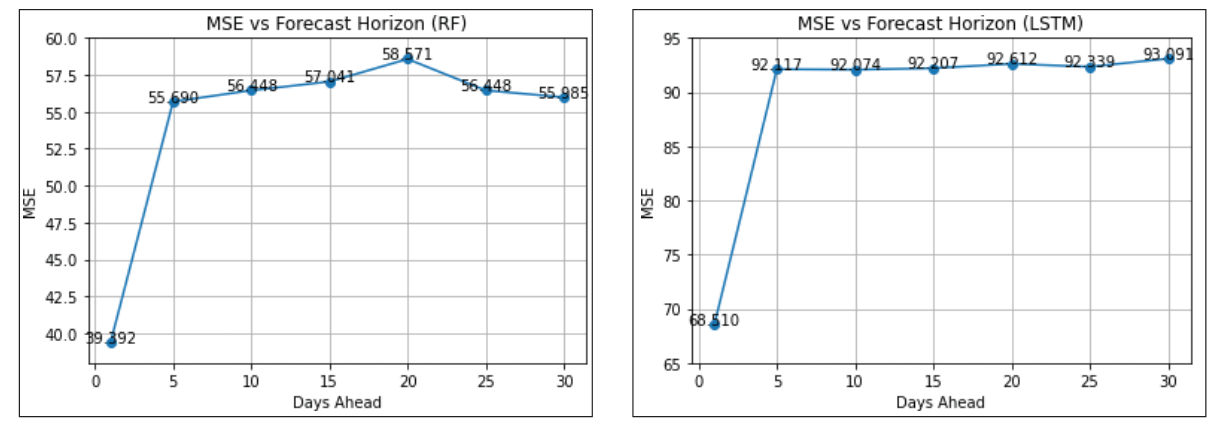
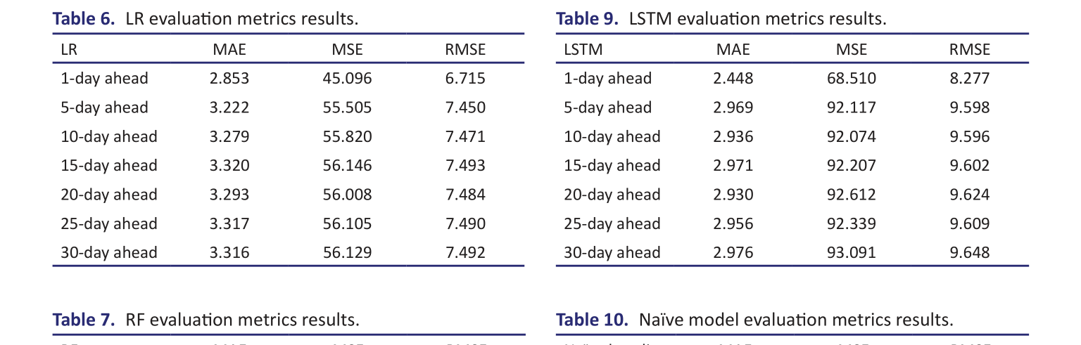
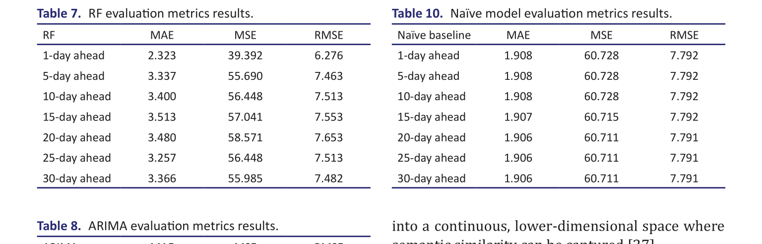
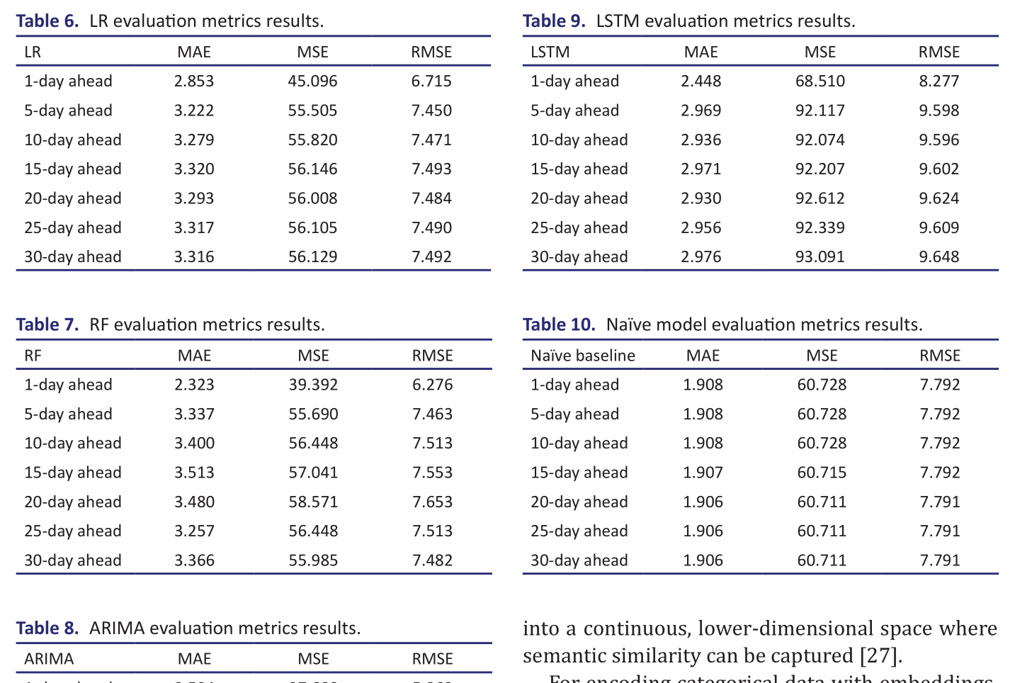
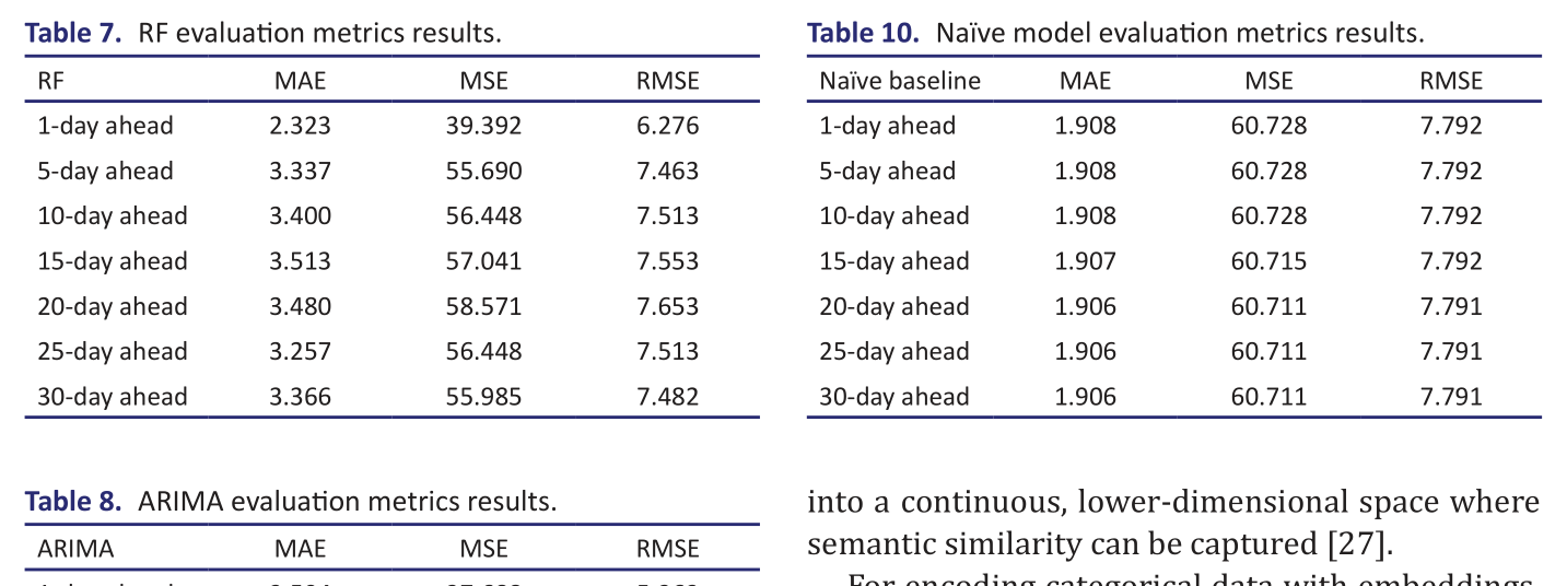
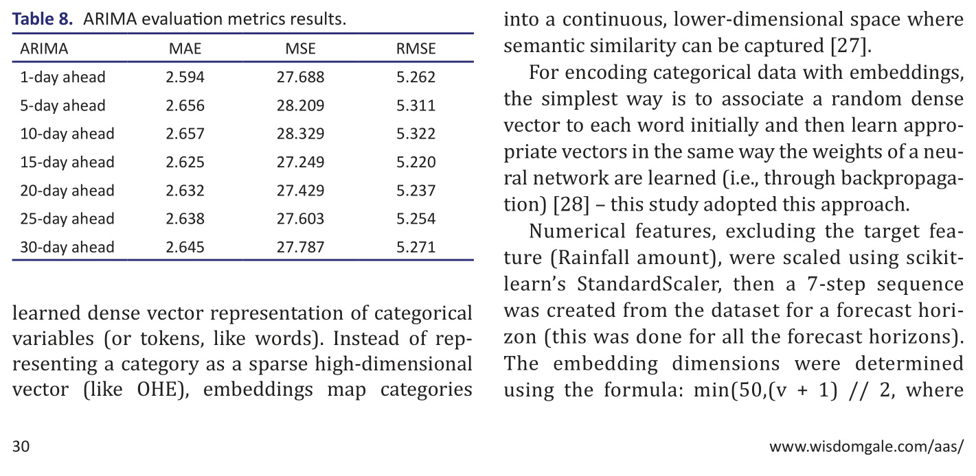
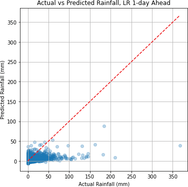
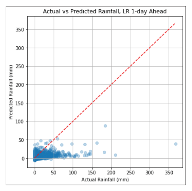
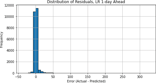
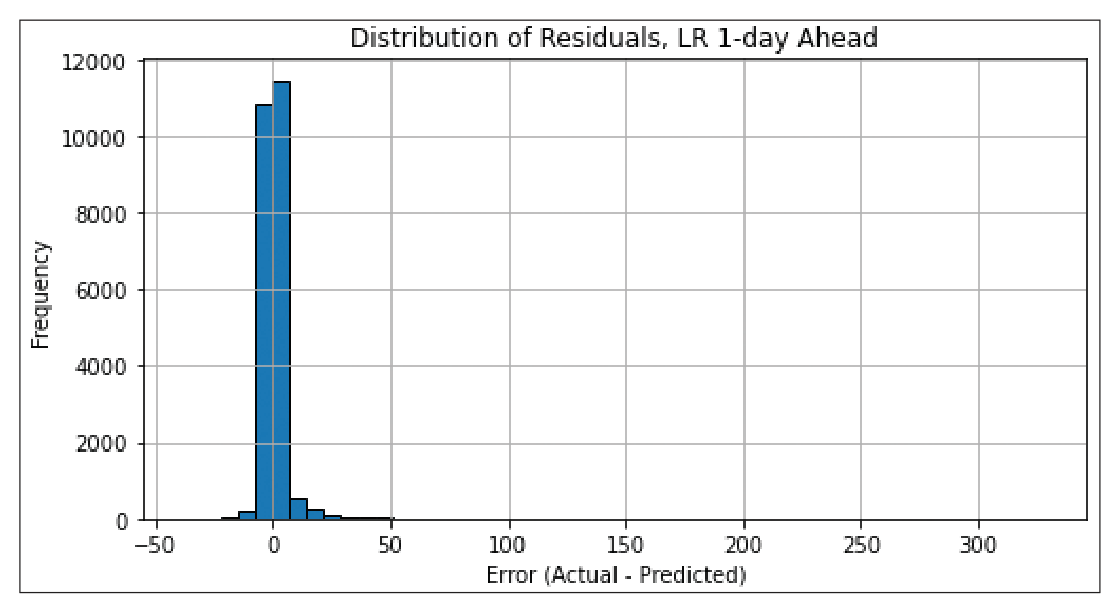
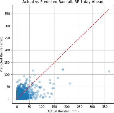
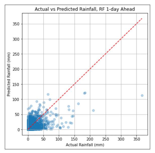
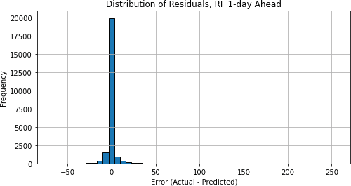
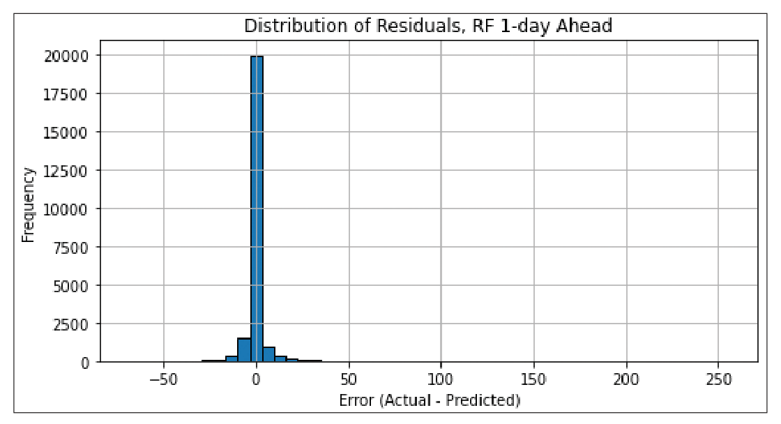
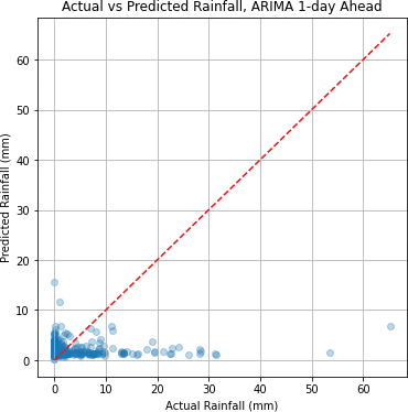
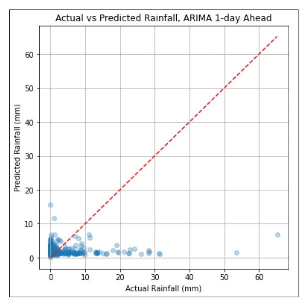
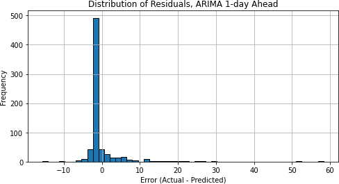
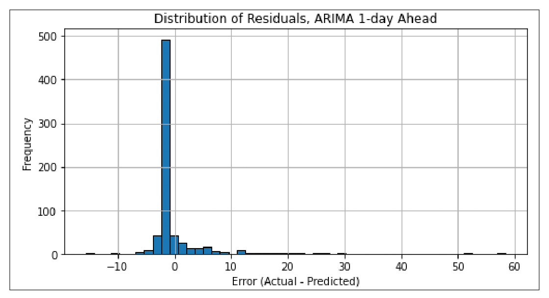
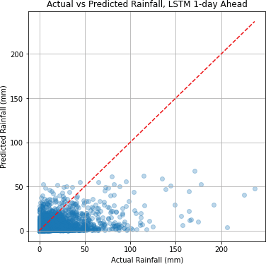
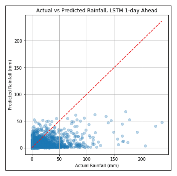
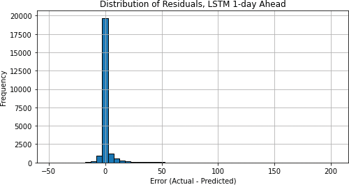
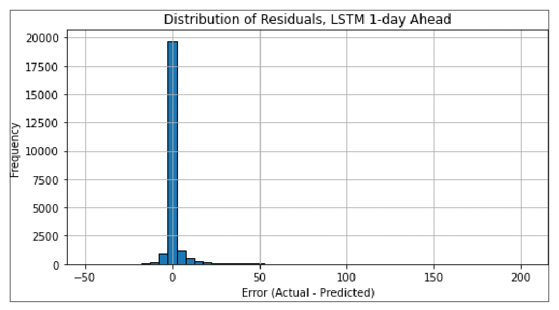
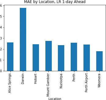
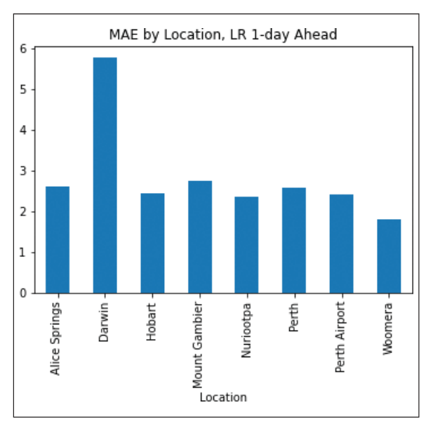
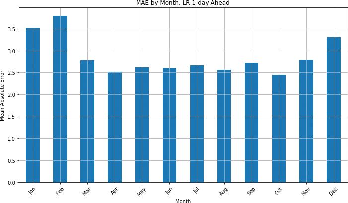
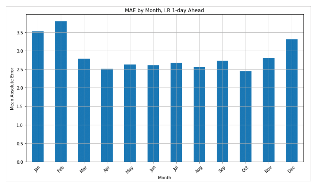
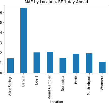
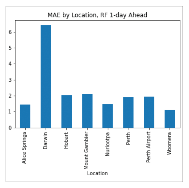
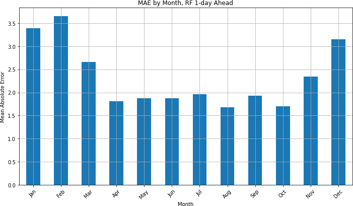
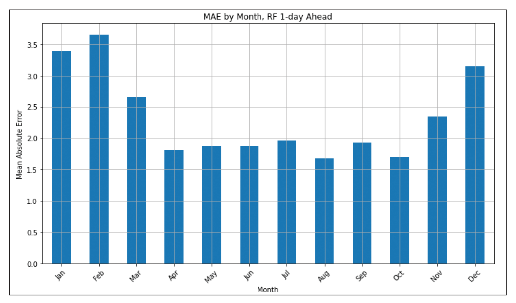
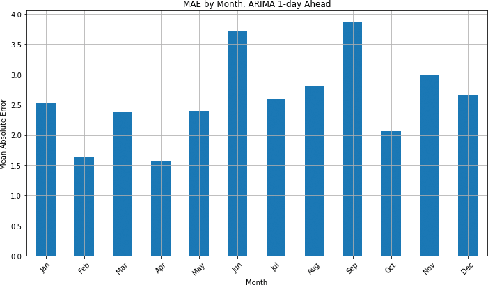
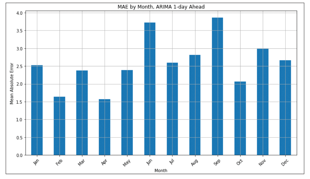
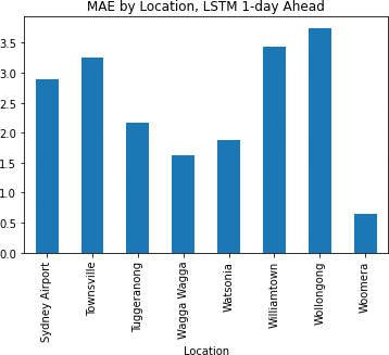
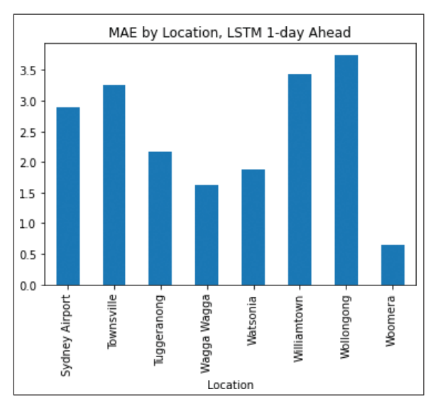
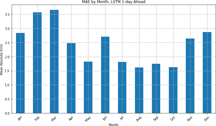
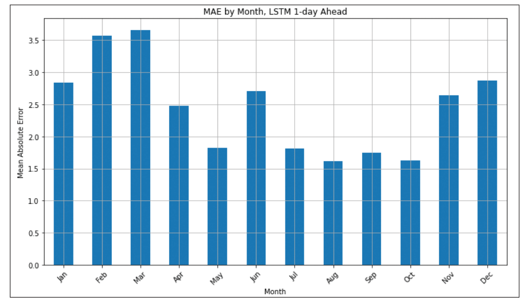
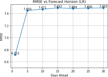
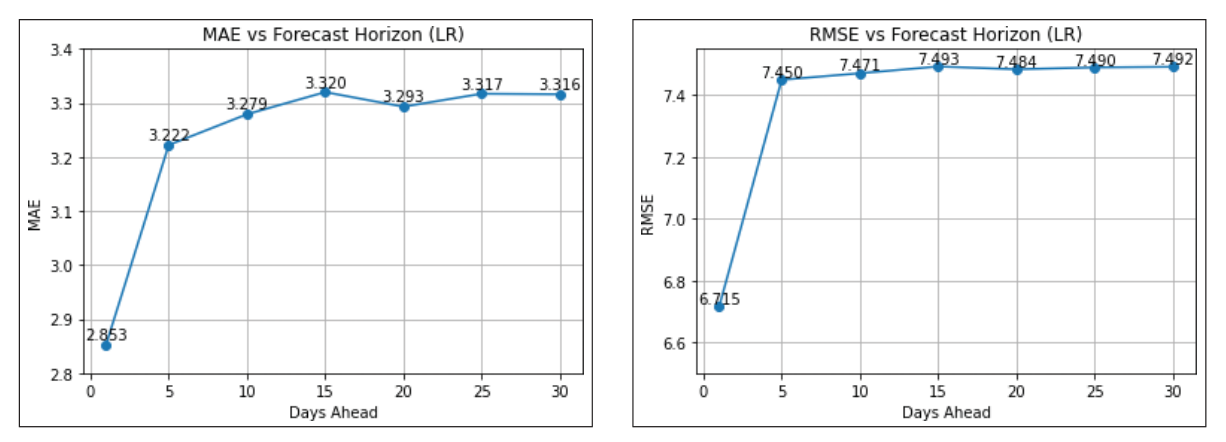
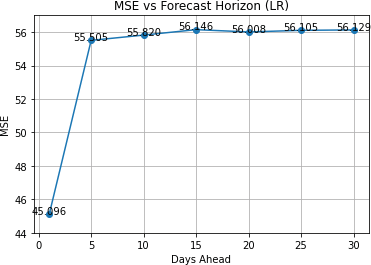
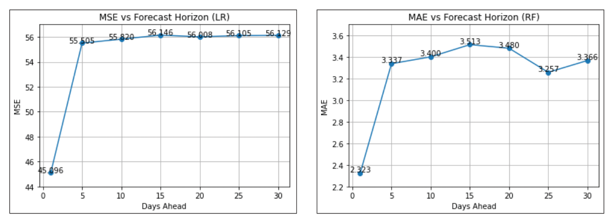
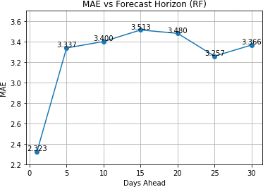
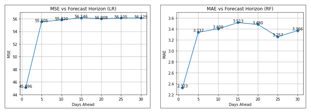
the four learned models LR, RF, ARIMA, and LSTM. Tables 6–10 report the MAE, MSE, and RMSE for each model (including the naïve baseline model) at the evaluated forecast horizons. The naïve baseline’s MAE is equal to the mean rainfall in the test set (1.908 mm): because rainfall is nonnegative, predicting 0 yields an absolute error equal to the observed value, so the baseline MAE equals the sample’s mean. From the tables, it can be observed that none of the learned models outperformed the naïve model in MAE across all horizons evaluated, which is unsurprising given the high proportion of zerorain days (the 50th percentile of rainfall amount is 0.0 mm). In contrast, many learned models (LR, RF, and especially ARIMA) beat the naïve model in MSE and RMSE across the horizons – with ARIMA performing best among the three models on squarederror metrics. LSTM had the largest MSE and RMSE values across all the horizons – indicating LSTM made some very large errors – although its MAE is competitive with the other learned models across all the horizons. ARIMA had the lowest (best) MAE among the learned models for almost every horizon (except 1-day ahead, where RF is best and LSTM is second). Overall, these results indicate that: (1) for overall daytoday error (MAE) a simple zero baseline can be hard to beat on very zeroinflated datasets; (2) ARIMA captures large rainfall events best (among the models evaluated); and (3) across nearly all forecast horizons, ARIMA consistently reduces absolute prediction errors compared to the other learned models. It should be noted, however, that the ARIMA model was trained and tested on only one location, while other models were trained on 31 locations and tested on 8 locations, which limits direct comparability.See Figures 4–11 for the actual versus predicted rainfall and residual distributions for the models. The actual versus predicted rainfall plots show that LSTM had more outliers to deal with, which was due to the fact that the dataset was sorted by location and date prior to creating sequences – making the locations used to train and test different from the ones used by RF and LR. Whereas, the residual distributions at 1-day ahead show that on most days the difference between the actual and predicted values were around 0 mm (especially so with RF and LSTM). Figures 12–18 show the MAE by location and month for the models. As RF and LR had the same test set, the plots of MAE by location indicate that they both had trouble predicting rainfall at location Darwin (both had MAE that were 5+ compared with other locations that were less than 3). It should also be noted that the three models (LR, RF, and LSTM) had the lowest MAE at location Woomera. The MAE by month plots showed a pattern in RF and LR: The MAE was highest in the months November – March. The pattern almost extended to LSTM, but June had an MAE higher than November, so it could be said that across the models that predict rainfall based on atmospheric features observed (LR, RF, and LSTM), the MAE was highest in the months December – March. The months December – March correspond to the summer season and early autumn. In particular, northern Australia (for example, Darwin and other tropical stations) experiences its monsoon / wet season in this interval, with much larger and more variable rainfall. This regional seasonality helps explain the elevated MAE observed in December–March for models that rely on atmospheric predictors: models must contend with rarer but much larger rainfall events during the wet season, which increases both average and extreme prediction errors. By contrast, locations such as Woomera (arid/semiarid

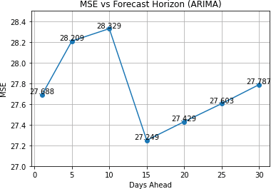
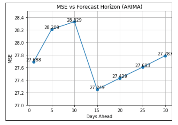
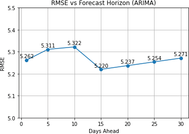
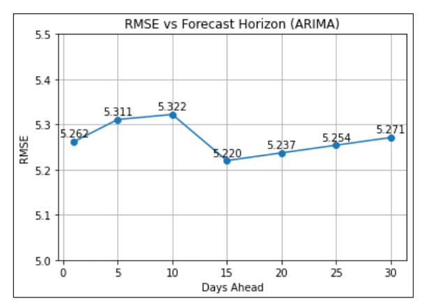
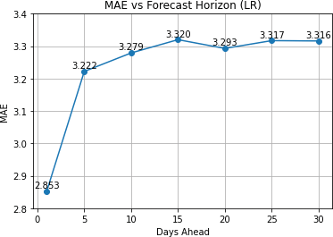
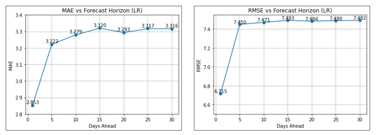
interior) show low MAE because they have far fewer wet days. This geographic heterogeneity in seasonal behavior underscores the need to report perlocation and permonth diagnostics (Figs. 12–18) and to consider location or climatezonespecific modelling strategies. Figures 19–30 show plots of evaluation metrics for all models (excluding the naïve model) across the forecast horizons.

Summary, Conclusion, and Suggestions for Further Study

Summary

This study focuses on predicting rainfall amounts in the study area using four modeling approaches –LR, RF, Autoregressive ARIMA, and LSTM – for forecasting daily rainfall amounts at multiple horizons (1, 5, 10, 15, 20, 25, and 30 days). A naïve baseline that predicts 0 mm daily was included for reference. The results show that: (i) no learned model outperformed the naïve baseline on MAE across all horizons, which is expected given the large fraction of zerorain days; (ii) many learned models (LR, RF, and especially ARIMA) had better MSE and RMSE results relative to the baseline, indicating handling of large rainfall events; (iii) LSTM produced the secondbest MAE across all horizons, but larger MSE and RMSE (indicating it produced some very large errors); (iv) perlocation and permonth diagnostics show pronounced geographic and seasonal heterogeneity: errors are largest in December–March (Australian summer/northern Australia wet season) and concentrated in tropical locations such as Darwin, while arid locations (e.g., Woomera) show low MAE due to far fewer wet days. The evaluation also revealed methodological caveats that affect interpretation: different models were trained/tested using slightly different data preparation choices (for example, ARIMA was trained on a single, longlocation time series while ML models were trained on multiple locations).

Conclusion

Predicting daily rainfall amount from meteorological features is challenging on this multilocation time series dataset because rainfall is heavily zeroinflated and spatially heterogeneous. A trivial predictor that always predicts zero achieves a low MAE because most days have zero rainfall – this sets a strong, simple benchmark that learned models must outperform on both occurrence and magnitude to be practically useful. The models’ comparability is limited by preprocessing (e.g., ARIMA trained on a single location versus ML models trained across many locations and LSTM tested on a set of locations that is different from LR and RF). For operational use (e.g., flood preparedness or irrigation scheduling), a singlestage regression that minimizes MAE is not sufficient. A practical forecasting system should (a) explicitly model occurrence and amount separately, and (b) evaluate conditional performance on wet days and extreme events.

Suggestions for further study

In future studies, it would be beneficial to (a) implement a twostage modeling, i.e., train a classifier for rain occurrence (rain/no rain) and a conditional regressor for rain amount only on rainy days – this would address zerorain inflation and improve results on wet days; (b) ensure all models use the same split (same locations for train and test), to make comparisons fair; (c) report conditional metrics, i.e., present evaluation metrics on (i) all days, (ii) rainy days only, and (iii) top quantiles of rainfall amount (e.g., top 1% events); and (d) group locations by climate zone and train specialized models.

References1. Rain. Wikipedia. San Francisco, CA. Available via https://en.wikipedia.org/wiki/Rain (Accessed 5 May 2022) 2. Warner K, Afifi T, Henry K, Rawe T, Smith C, de Sherbinin A. Fact sheetwhere the rain falls: climate change. Food and Livelihood Security, and Migration, UN, New York City, NY, 2013 [Online]. Available via https://www.un.org/en/development/desa/population/events/pdf/11/20130212warneretalclimatechangefoodsecuritymigration_facts.pdf3. United States Environment Protection Agency. Climate Change Indicators. Available via https://www.epa.gov/climateindicators (Accessed 11 May 2022) 4. Swain S, Patel P, Nandi S. A multiple linear regression model for precipitation forecasting over Cuttack district, Odisha, India. Presented at I2CT’17 [Online]; doi: 10.1109/I2CT.2017.82261505. Graham S, Parkinson C, Chahine M. Weather forecasting through the ages. NASA, Washington, DC, 2002 [Online]. Available via https://earthobservatory.nasa.gov/features/WxForecasting/wx2.php6. Boscher L, Chmutina K. Windstorms [Online]. In: Disaster risk reduction for the built environment, Wiley, Chichester, UK, 4, p 103, 2017. Available via https://onlinelibrary.wiley.com/doi/book/10.1002/9781119233015 7. Barrera-Animas AY, Oyedele LO, Bilal M, Akinosho TD, Delgado JMD, Akanbi LA. Rainfall prediction: a comparative analysis of modern machine learning algorithms for timeseries forecasting. Mach Learn Appl 2022; 7:100204.

8. Paras SM. A simple weather forecasting model using mathematical regression. Indian Res J Ext Edu 2016; 12:161–8. 9. Terzi O. Monthly rainfall estimation using datamining process. Comput Intell Soft Comput 2012; 2012:698071; doi:10.1155/2012/698071 10. Olatayo TO, Taiwo AI. Statistical modelling and prediction of rainfall time series data [Online]. Global J Comput Sci Technol 2014; 14(1):1–9. Available via https://globaljournals.org/GJCST_Volume14/1-Statistical-Modellingand-Prediction.pdf 11. Hasan N, Nath C, Rasel IR. A support vector regression model for forecasting rainfall. In 2nd International Conference on Electronics and Integrated Circuit Technology, Khulna, Bangladesh, 2015, pp. 554–9; doi:10.1109/EICT.2015.7392014 12. Zainudin S, Jasim DS, Abu Bakar A. Comparative analysis of data mining techniques for malaysian rainfall prediction. Int J Adv Sci Eng Inf Technol 2016; 6(6):1148–53. 13. Prabakaran S, Kumar PN, Sai P, Tarun M. Rainfall prediction using modified linear regression [Online]. ARPN J Eng Appl Sci 2017; 12(12):3715–8. Available via https://www.arpnjournals.org/jeas/research_papers/rp_2017/jeas_0617_6115.pdf 14. Tharun VP, Prakesh R, Devi SR. Prediction of rainfall using data mining techniques. In Proceedings of 2nd ICICCT, IEEE (Institute of Electrical and Electronics Engineers), Coimbatore, India, 2018, pp. 1507–12; doi:10.1109/ICICCT.2018.8473177 15. Vijayan R, Mareeswari V, Mohankumar P, Gunasekaran G, Srikar K. Estimating rainfall prediction using machine learning techniques on a dataset [Online]. Int J Sci Technol Res (New Delhi) 2020; 9(6):440–5. Available via https://ijstr.org/finalprint/jun2020/Estimating-Rainfall-Prediction-Using-Machine-Learning-Techniques-On-A-Dataset.pdf 16. Liyew CM, Melese HA. Machine learning techniques to predict daily rainfall amount [Online]. J Big Data 2021; 8(153):1–10; doi:10.1186/s40537-021-00545-4 17. Alakh S. One hot encoding vs label encoding using scikitlearn. Analytics Vidya, Wilmington, DE, 2023 [Online]. Available via https://www.analyticsvidhya.com/blog/2020/03/onehotencodingvslabelencodingusingscikitlearn/ (Accessed 18 March 2024) 18. Indraneel D. All you need to know about encoding techniques. ANOLYTICS, Levittown, NY, 2023 [Online]. Available via https://medium.com/anolytics/allyouneedtoknowaboutencodingtechniquesb3a0af68338b (Accessed 18 March 2024) 19. Wojtek F. Onehot encoding — a brief explanation. Medium, San Francisco, CA, 2023 [Online]. Available via https://medium.com/ [at] WojtekFulmyk/onehotencodinga-briefexplanation-8c5daec395e3 (Accessed 18 March 2024)20. Sharma N. One hot encoding using categorical data. Analytics Vidhya, Wilmington, DE, 2024 [Online]. Available via https://www.analyticsvidhya.com/blog/2023/12/howtodoonehotencoding/ (Accessed 19 March 19 2024) 21. Lekhana G. One hot encoding in machine learning. GeeksforGeeks, Noida, India, 2023 [Online]. Available via https://www.geeksforgeeks.org/mlonehotencodingofdatasetsinpython/ (Accessed 19 March 2024) 22. Lewinson E. Three approaches to encoding time information as features for ML models. NVIDIA Technical Blog, Santa Clara, CA, 2022. Available via https://developer.nvidia.com/blog/threeapproachestoencodingtimeinformationasfeaturesformlmodels/ (Accessed 31 August 2025) 23. MacKenty B. Mean absolute error (MAE). Computer Science Wiki, 2022 [Online]. Available via https://computersciencewiki.org/index.php/Mean_absolute_error_(MAE) (Accessed 20 February 2023)24. Radial basis function. Wikipedia, San Francisco, CA. Available via https://en.wikipedia.org/wiki/Radial_basis_function (Accessed 31 August 2025)25. Cyclical features in time series. Skforecast Docs. Available via https://skforecast.org/0.17.0/faq/cyclicalfeaturestimeseries (Accessed 31 August 2025)26. Brownlee J. Ordinal and onehot encodings for categorical data. MachineLearningMastery, San Juan, PR, 2020. Available via https://machinelearningmastery.com/onehotencodingforcategoricaldata/ 27. Word embeddings. TensorFlow, Mountain View, CA. Available via https://www.tensorflow.org/text/guide/word_embeddings (Accessed 01 September 2025)28. Chollet F. Deep learning with python. In: Arritola T, Gaines J, Dragosavljevic A, Taylor T (eds.). Deep learning with python, Manning Publications Co., Shelter Island, NY, p 184, 2018. 29. Hyndman RJ, Athanasopoulos G. Forecasting: Principles and Practice, 2nd Edition, OTexts, Melbourne, Australia, 3, pp 80–1, 2018.30. Gupta A. Mean squared error: overview, examples, concepts and more. Simplilearn, Plano, TX, 2023 [Online]. Available via https://www.simplilearn.com/tutorials/statisticstutorial/meansquarederror (Accessed 20 February 2023)31. Gunjal S. What is root mean square error (RMSE). Kaggle, Mountain View, CA, 2021 [Online]. Available via https://www.kaggle.com/general/215997 (Accessed 20 February 2023)32. Project Jupyter. Home. Available via https://jupyter.org/ (Accessed 23 February 2023)